Frequently Asked Questions

How does the CABS-flex method work?

The CABS-flex 3.0 web server is designed to operate in two distinct modes: Flexibility Modeling and Peptide Modeling, see pipeline below.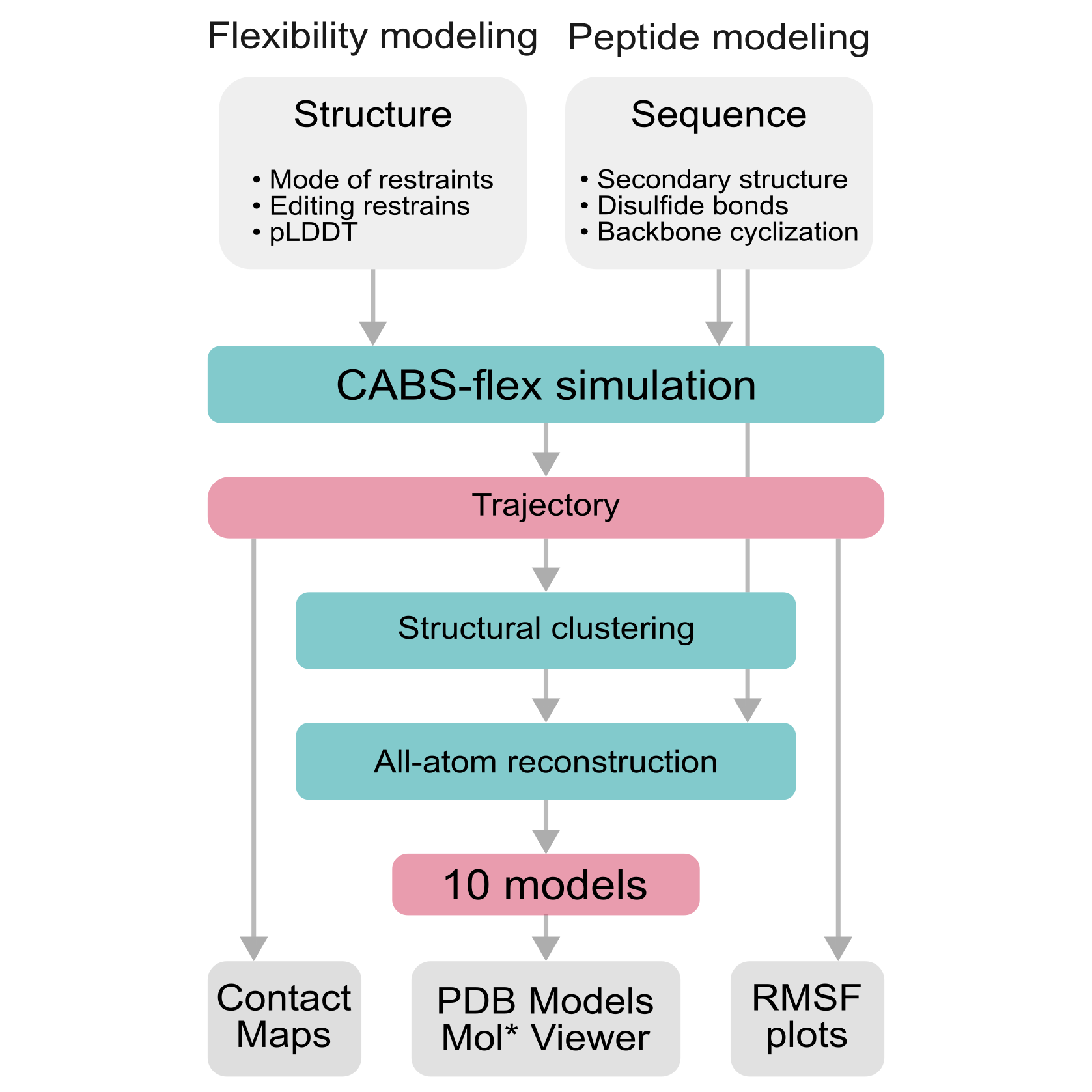 Flexibility modeling uses multiscale modeling pipeline merging CABS coarse-grained model with all-atom reconstruction, see [CABS-flex 3.0 paper in review and Protein Sci 2024]. Peptide modeling uses modeling protocol described in [Brief in Bioinfo 2024].

How to run flexibility modeling?

To begin a flexibility modeling simulation, you need to provide a protein structure in PDB format. You can do this in two ways:

• Enter a PDB ID – If your structure is available in the Protein Data Bank (PDB), enter its four-character code in the "PDB code/PDB file" box.
• Upload a PDB file – If you have the file on your computer, click “Browse” to locate and upload it.

The only required input is the protein structure. Other optional but important settings include:

• Flexibility mode – Pay attention to this setting, as it determines the extent of structural fluctuations in the simulation. The default option is Rigid, but you can change it as needed. More details: [How to use flexibility mode?]
• Residue-level flexibility control – Modify flexibility for specific protein fragments. See: [How to modify residue-level flexibility?]
• Project name – Helps identify your job. If left blank, a random hashcode is assigned.
• Chain selection – Choose specific chains from the uploaded PDB file.
• Email notification – Get an email when the job is completed.
• Privacy option – Enable “Do not show my job on the results page” to keep it private (accessible via a direct link only).

The following screenshot shows the main page along with the discussed input options. For additional customization, see: [How to use advanced simulation options?]

Once all parameters are set, click "Run" to start your simulation.

How to use flexibility mode?

CABS-flex 3.0 introduces flexibility modes, which allow users to control how much different parts of the protein can move. These modes define the range of residue movements by applying different distance restraint schemes:

• Flexible mode applies distance restraints only to residues forming secondary structure elements, allowing greater flexibility in loops and unstructured regions. Previously referred to as ‘SS2’ in earlier versions of CABS-flex 2.0 [Nucleic Acids Res 2018] and standalone application [Bioinformatics 2019], it provides a balanced representation of protein dynamics. This mode has been validated against crystallographic B-factors and atomistic MD simulations using various force fields [J Chem Theory Comput 2013], NMR ensembles [Bioinformatics 2014], as well as in numerous structure–flexibility-function studies supported by experimental evidence, including Cryo-EM–derived conformational variability and functional analyses related to aggregation propensity and S-nitrosylation sensitivity [Protein Sci. 2024]. Importantly, the ability of the CABS model to predict loop structures ab initio has been demonstrated across various protein systems [BMC Struct. Biol. 2010, Biophys. J. 2014], including in the context of peptide interactions [Methods 2016], highlighting its suitability for modeling local structural variability.
• Rigid mode imposes uniform restraints on all residues, minimizing fluctuations throughout the structure. Equivalent to the ‘All’ mode described previously ([Nucleic Acids Res 2018, Bioinformatics 2019], it effectively preserves native-like conformational constraints. Benchmarking with CHARMM36m-based ATLAS MD simulations showed high correlation with MD-derived fluctuation profiles, particularly in structured, globular proteins [Comput Struct Biotechnol J 2024]. It is worth noting that the selection criteria of the ATLAS dataset favor well-folded, high-resolution monomeric proteins, which may bias the dataset toward more structurally stable and less flexible systems. However, some degree of intrinsic flexibility is still likely present in the selected structures.
• Rigid-pLDDT mode improves flexibility predictions by integrating structural confidence into the simulation process. In this mode, restraint strength is modulated according to per-residue pLDDT scores and secondary structure classification, as introduced in our recent work [Comput Struct Biotechnol J 2024]. It is applicable when pLDDT scores are available, as in AlphaFold-predicted structures. Users may supply pLDDT values either through the B-factor field in the PDB file or via an external .json or .tsv file. Based on general observations, the overall level of flexibility generated by this mode tends to be closer to Rigid than Flexible, which is reflected in the naming convention, and the mode has been validated using ATLAS MD simulation data [Comput Struct Biotechnol J 2024].
• Unleashed mode applies no restraints, allowing for fully unrestricted conformational sampling. The resulting ensemble is governed solely by the intrinsic properties of the CABS coarse-grained force field. This mode is designed as an advanced option, recommended primarily for exploratory simulations where it is important to observe the behavior of a system in the complete absence of restraints. While this mode typically shows lower agreement with MD-derived fluctuation profiles and may produce exaggerated motions, it is valuable for modeling folding/unfolding processes or large-scale transitions in disordered or flexible systems. In such cases, meaningful results may require careful tuning of additional simulation parameters, such as temperature and number of cycles. The applicability of CABS-based simulations to disordered and unfolded protein systems has been reviewed in our previous work [Int. J. Mol. Sci. 2019], which discusses several case studies involving disordered binding partners and unstructured regions.

By default, Flexible mode is enabled in CABS-flex 3.0 due to its versatility and proven accuracy. For stable, well-folded proteins, the Rigid mode may be most appropriate. When pLDDT scores are available, we recommend using Rigid-pLDDT, which incorporates structural confidence into simulations and improves predictive accuracy. Conversely, for systems expected to undergo large-scale motions or unfolding, the Unleashed mode can be used, with caution and additional parameter tuning. When in doubt, we recommend running simulations with multiple flexibility modes, particularly Rigid, Flexible, and Rigid-pLDDT, and comparing the resulting fluctuation profiles with available structural or functional knowledge about the protein. This comparative approach can help identify the most appropriate mode for a given system. Examples of using each individual mode are illustrated in the Gallery.

CABS-flex 3.0 also offers a residue-level flexibility editor that allows users to manually assign flexibility categories prior to simulation. This option is further described in section: How to modify residue-level flexibility?

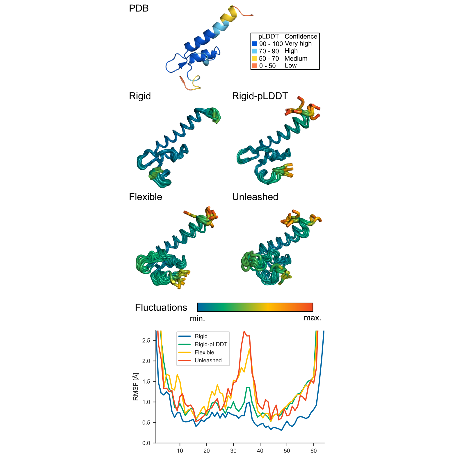
The image below illustrates an example effect of distance restraint modes on backbone fluctuations in the simulation. It shows, from the top left, the starting protein structure (PDB ID: 2f60 chain K) colored by pLDDT, followed by output structures generated using different restraint modes: Rigid, Rigid-pLDDT, Flexible, and Unleashed. Further details on these restraints were recently discussed in [Comput Struct Biotechnol J 2024].

How to use advanced simulation options in flexibility modeling?

Advanced options allow users to modify default settings based on their needs and available information about the modeled system.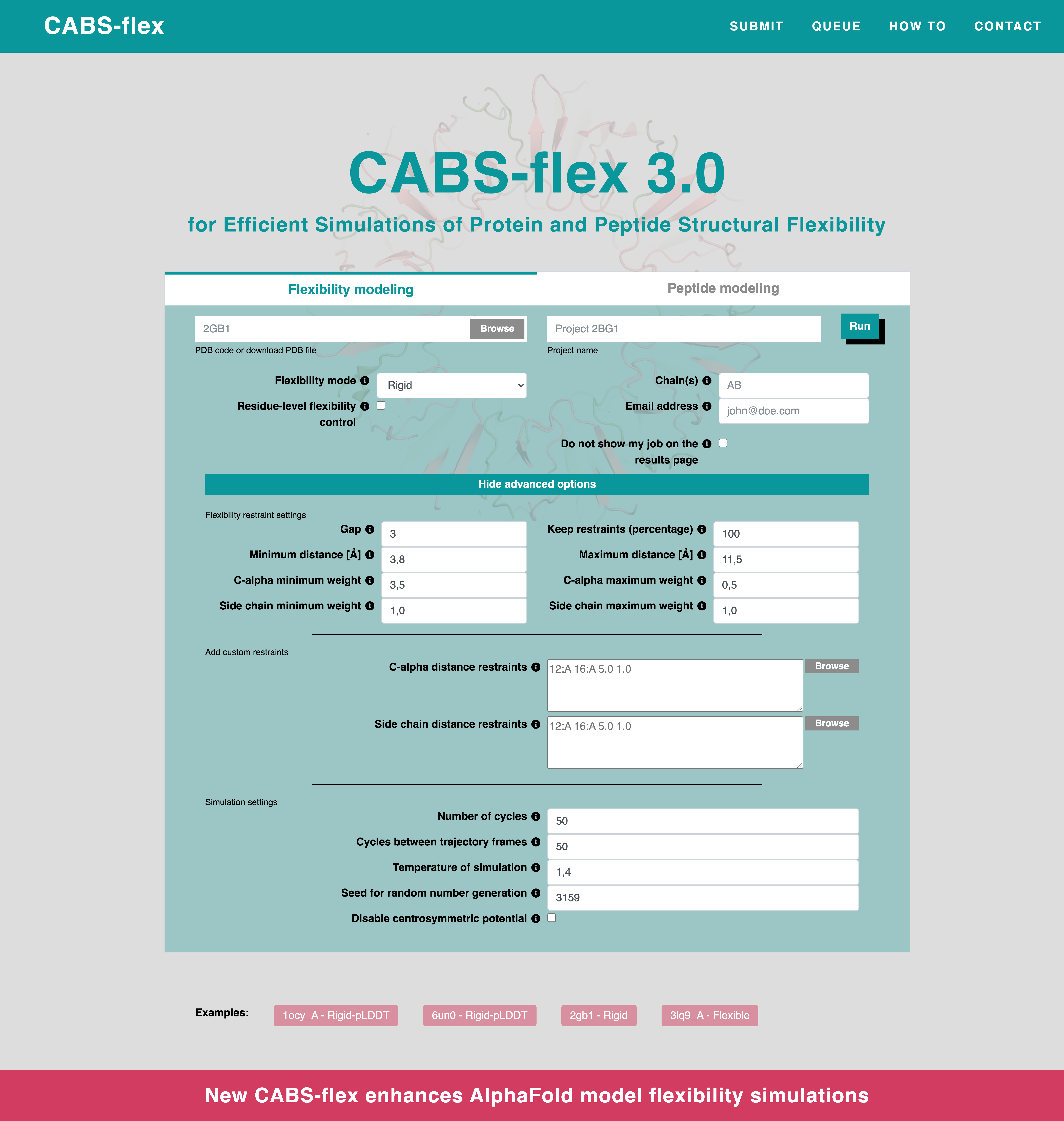 The options can be split into three distinct section, which are:

Flexibility Restraint Settings

These options refer mostly to automatically generated restraints (What are protein restraints?) according to the scheme defined by the Flexibility Mode (How to use flexibility mode?).

Gap sets the minimum distance along the protein sequence for two residues to be bound with a restraint. By default, Gap is equal to 3, which means for example that residue number 15 cannot be restrained with residues numbered from 12th to 18th.

Minimum and Maximum set the allowed restraint length in Angstroms. The restraints will be automatically generated only if the two residues are within these distances. By default Minimum is 3.8 Å and Maximum is 11.5 Å.

Keep restraints allows reducing the number of automatically generated restraints indicating the percentage of restraints to keep. This option can be used in order to increase flexibility. The number must be between 100 and 0. Restraints are randomly removed so that the final number of restraints N_final = N_all × (PERCENTAGE ÷ 100).

Finally, there are four fields related to restraint weights: CA restraints and side chain restraints. In the CABS model, these restraints add to the total simulation energy when the distance between restrained residues goes beyond a set limit. The higher the restraint weight, the greater the energy penalty. There are two types of weights: Minimum weight, applied when the distance is too small, and Maximum weight, applied when the distance is too large. The weights value must be non-negative, but value equal to 0 makes the restraints non-existent.

Custom Restraints

Besides the automatically generated restraints, the users can input their own restraints imposed on the modeled protein structure. The top panel is for the Cα–Cα restraints and the bottom panel is for the side chain–side chain restraints (SC–SC). Restraints can be added either through the text box or from an uploaded text file. The restraints are defined by the following syntax: “residue1_id residue2_id distance weight”, for example:
“123:A 73:B 12.5 1.0”.
This example defines a single restraint between the 123th residue of chain A and the 73rd residue of chain B to be at a distance of 12.5 Å with a restraint weight of 1.0.

Simulation Settings

This panel enables modification of the parameters that control the simulation.

Number of cycles (Ncycle) sets the total number of models saved in the trajectory to be equal to 20 x Ncycle. For example, setting Ncycle = 50 results in 20 × 50 = 1000 models in the trajectory.

Cycles between trajectory frames (Nskipped), sets the number of models skipped on saving models. For example, when Nskipped = 100 every hundredth model will be saved. This field also indirectly sets the total number of models generated, i.e. for Ncycle = 50 and Nskipped = 100, the total number of generated models equals 20 × 50 × 100 = 100,000. However only 1000 of them will be written to the trajectory.

Temperature of simulation (T) is a dimensionless value that controls how much movement occurs in the system. Read more about the temperature in the section below: How to use and interpret CABS-flex temperature?

Seed for random number generation initializes the random number generator. This can be used to ensure reproducibility of the simulation. If the same seed is used, the same trajectory will be generated.

Disable centrosymmetric potential turns off the centrosymmetric potential in the CABS model, which pulls residues toward the center of the modeled protein. This can be useful for modeling large complexes or proteins with a high degree of disorder.

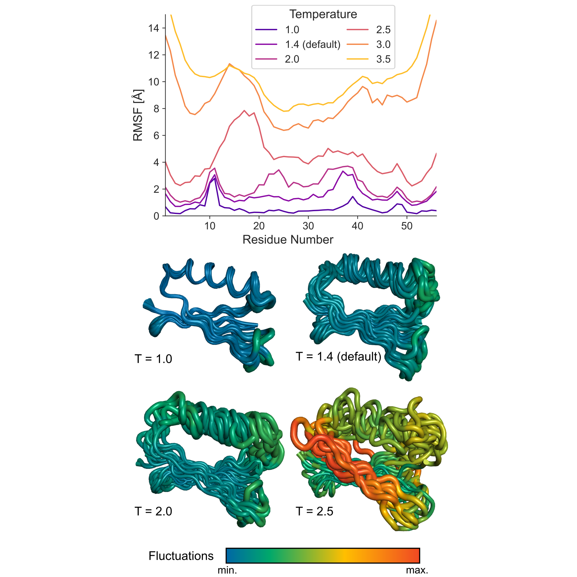
How to use and interpret CABS-flex temperature?

In CABS-flex, the temperature setting controls how flexible the simulated structure is. You can think of it as a slider for structural mobility: the higher the temperature, the more the protein can move during the simulation.

Although it's called "temperature", this value is not expressed in Kelvins and does not correspond directly to physical temperature. Instead, it is a dimensionless parameter used in the underlying Monte Carlo simulation algorithm to control the balance between structural stability and flexibility. The value affects how easily the model explores alternative conformations—higher temperatures allow for broader movement and more energetic transitions, while lower temperatures keep the structure closer to the starting model.

A common question from users is: “How can I convert the CABS-flex temperature to Kelvins?”

The answer is: you can’t—CABS-flex uses reduced temperature, a concept from statistical physics, which has no direct conversion to physical units. It simply scales how much conformational space the model explores.

The default temperature is T = 1.4, which works well for most typical applications, offering a balance between realistic fluctuations and overall structural integrity. If you're studying subtle flexibility or near-native dynamics, this default is usually appropriate. For more extensive motions—such as protein unfolding, large conformational changes, or modeling intrinsically disordered regions (IDPs)—you can try increasing the temperature to values like 1.6 or 2.0.

This behavior reflects how temperature is used in the underlying CABS coarse-grained model, where it plays a central role in balancing energetic preferences and conformational entropy.

The figure below shows how different temperature values affect the flexibility of protein G, a small globular protein (PDB ID: 2gb1), simulated using the Unleashed mode. In this mode, no distance restraints are applied, so the conformational sampling is driven solely by the internal force field of the CABS model. As illustrated, higher temperatures lead to global fluctuations in the range of approximately 8–15 Å, demonstrating the impact of temperature on conformational mobility.

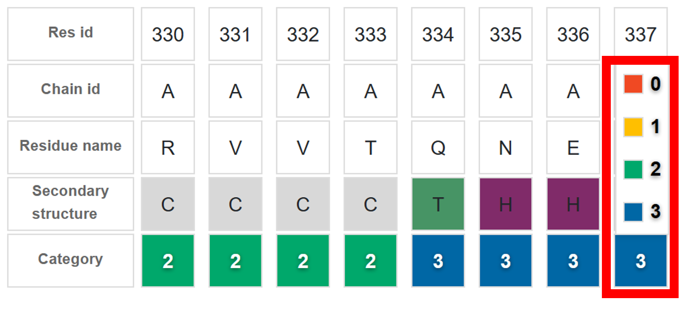
How to use Residue-level flexibility control?

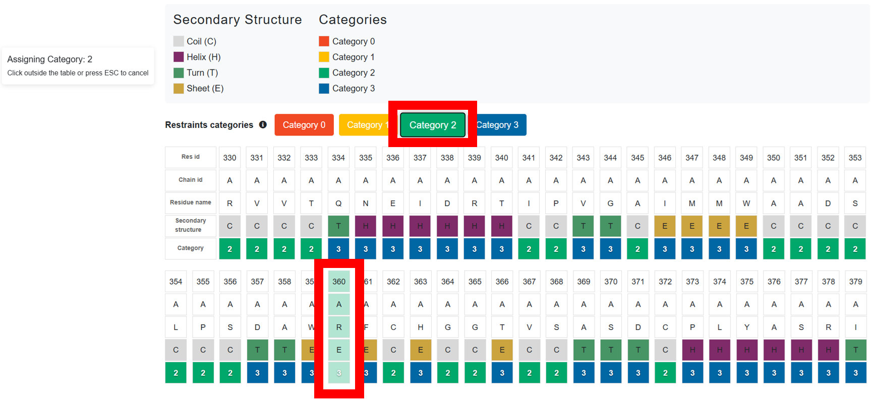
After selecting the Residue-level flexibility control checkbox during job submission, you are redirected to a dedicated page where you can manually adjust the flexibility level for each amino acid.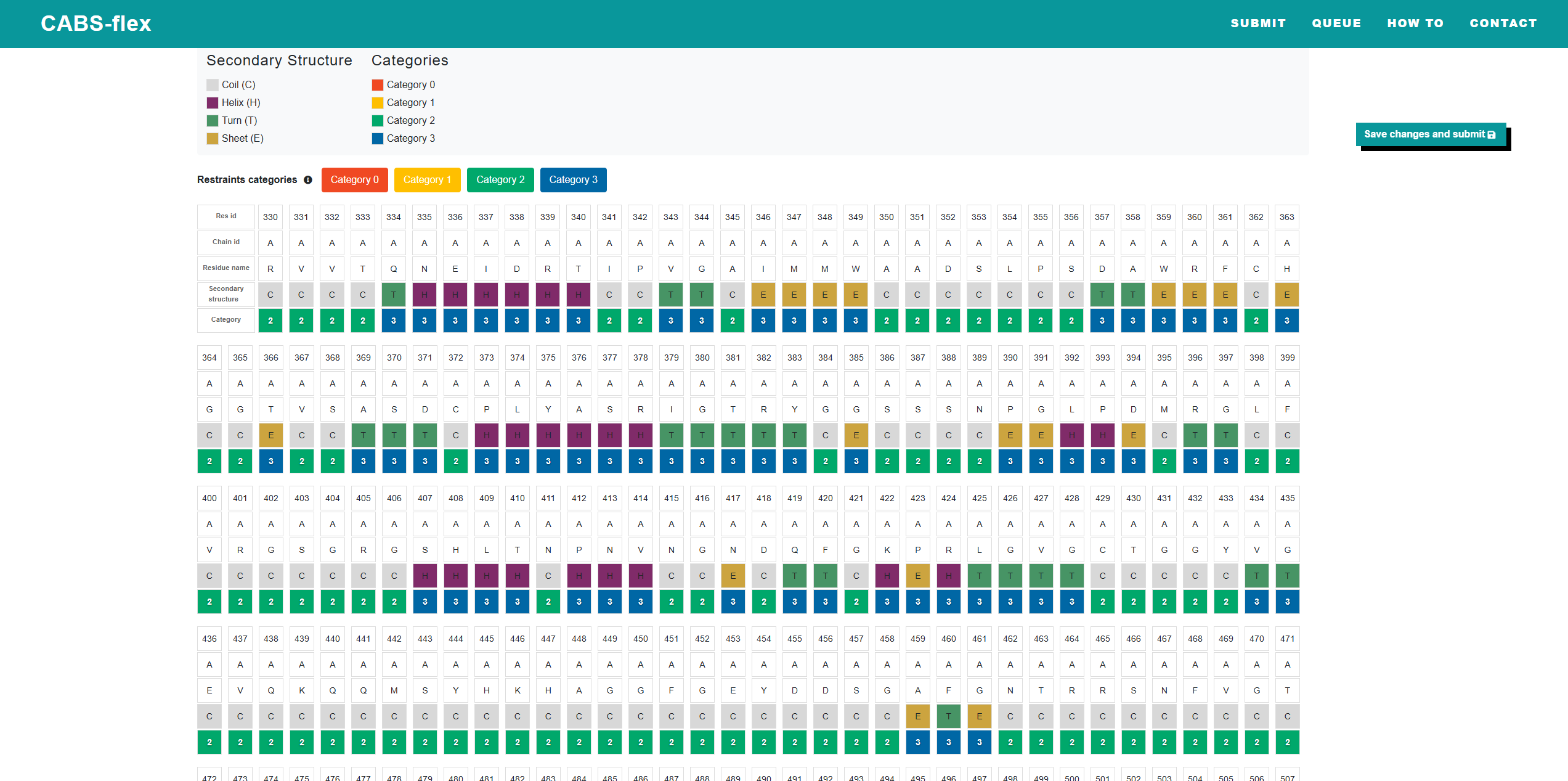 On this page, a table displays every residue from the sequence with the following details:

• Residue ID
• Chain ID
• Residue Name
• Secondary Structure
• Distance Restraint Category

Both the secondary structure and the restraint categories are color-coded, with legends at the top of the page explaining the color schemes. Each residue is initially assigned a distance restraint category:

• 3: Strong rigidity and tight structural bonds to the input
• 2: Weaker restraints
• 1: Intermediate flexibility
• 0: Full flexibility

To modify the category you can click on the category for the desired residue and select a new category from the dropdown. To modify multiple categories at once click one of the buttons labeled "category 0", "category 1", "category 2", or "category 3". Then, click on multiple residues to update their category simultaneously. To exit this multi-select mode, simply click outside the table or press the Esc key. Once you are satisfied with your changes, click "save changes and submit" to proceed with your job.

How to run peptide modeling?

To start a peptide modeling simulation, you need to provide a peptide sequence in the "Sequence" text box.

Once you've entered the sequence, click the “Run” button to submit your job. 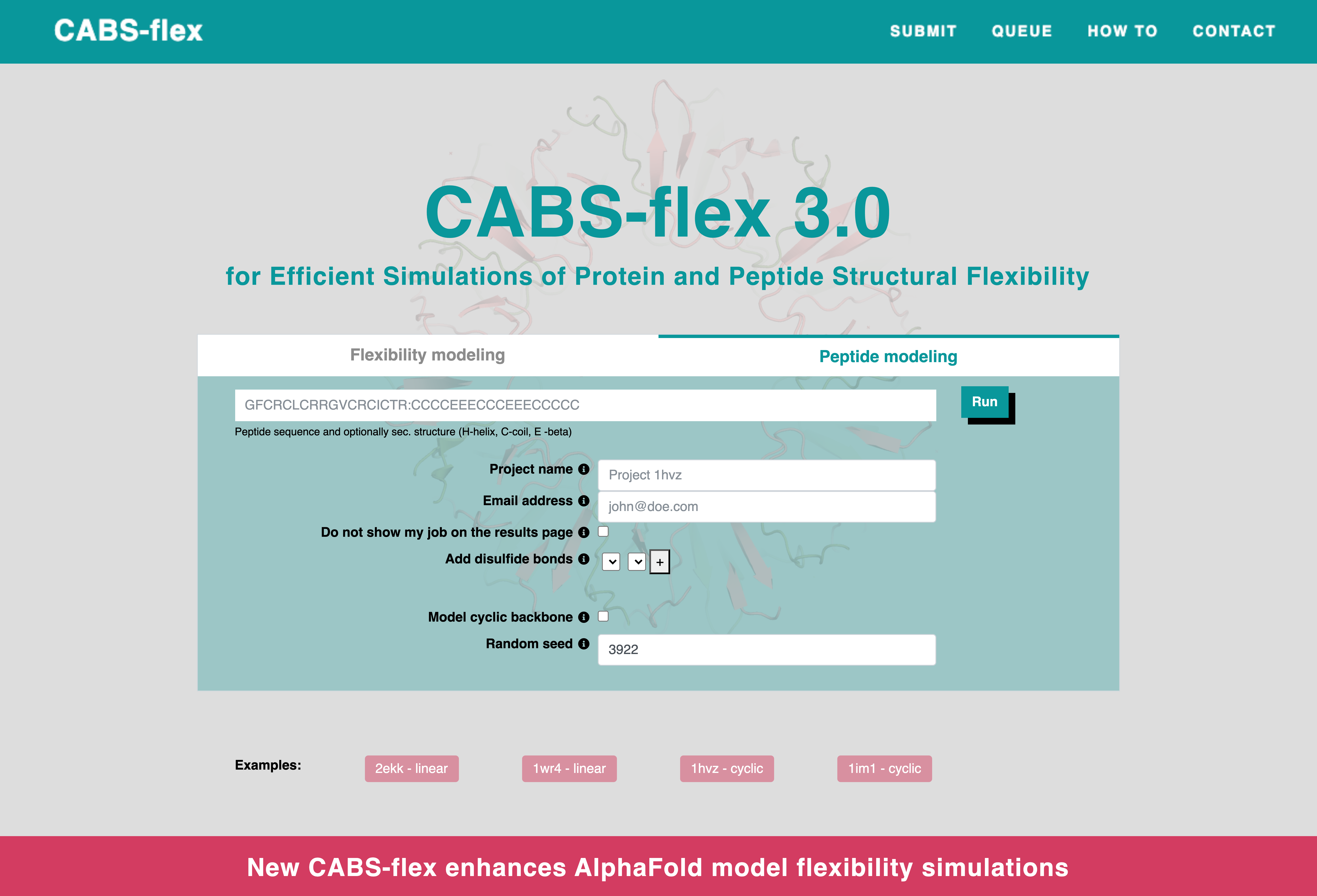Additionally, you can provide secondary structure information in HEC format (H = helix, E = beta-strand, C = coil) by entering it alongside the sequence, separated by a colon. For example: ALALA:CHHHH. If no secondary structure is provided, it will be predicted automatically using NetSurf-P 3.0 [https://services.healthtech.dtu.dk/services/NetSurfP-3.0/].

If you want to model cyclic peptides, you can do this in two ways:

• Add disulfide bonds enables adding disulfide bonds between selected cysteine residues. Pairs of cysteines, numbered according to the input sequence, can be specified and bonded by clicking the "+" button.
• Model cyclic backbone allows closing the backbone of the modeled peptide into a cyclic structure.

Peptide modeling uses methodology described in [Brief in Bioinfo 2024].

The other options are mostly used to help with handling jobs. All these inputs are optional and they include:

• Project name, which can help you find your job in the queue list. If not provided, the name will be replaced with a random hashcode. Chain(s), can be used if you want to select only specific chain(s) from the uploaded PDB file.
• Email address, which will be used by the server to send an email notification about job completion.
• Do not show my job on the results page will hide the job from the results page. You can still access the results via the direct link provided after submission.

How to analyse flexibility modeling?

When you initiate a new job in CABSflex 3.0, the interface starts with a single Project Information tab. This tab is split into two sections: the upper section shows basic project details along with buttons to download the input structure and output files, while the lower section provides in-depth details such as rigidity, restraints, and simulation parameter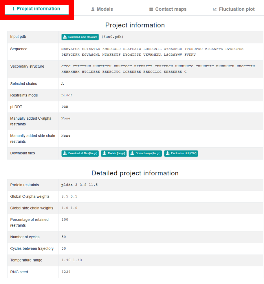s. 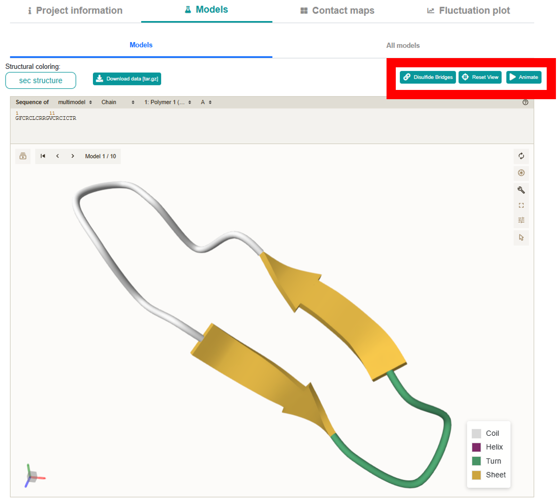After job completion, the page expands to include three additional tabs – Models, Contact Maps, and Fluctuation Plot – each designed to help you explore different aspects of the flexibility modeling results.

Models section leverages the interactive mol* viewer for 3D visualization and is organized into three sub-tabs:

• Structure:
  Loads by default to display the starting conformation. It offers a “Flexibility coloring:” dropdown (with options such as RMSF, pLDDT, and B-factor) and a “Structural coloring:” dropdown (allowing you to color the model by sequence, chain, secondary structure, or choose a custom monochrome color via a color picker).
• Models:
  Displays each of the 10 output models one at a time with next/previous navigation. It also supports the same “Structural coloring:” options.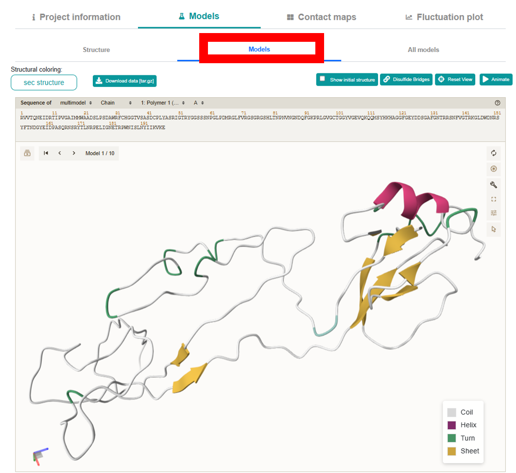
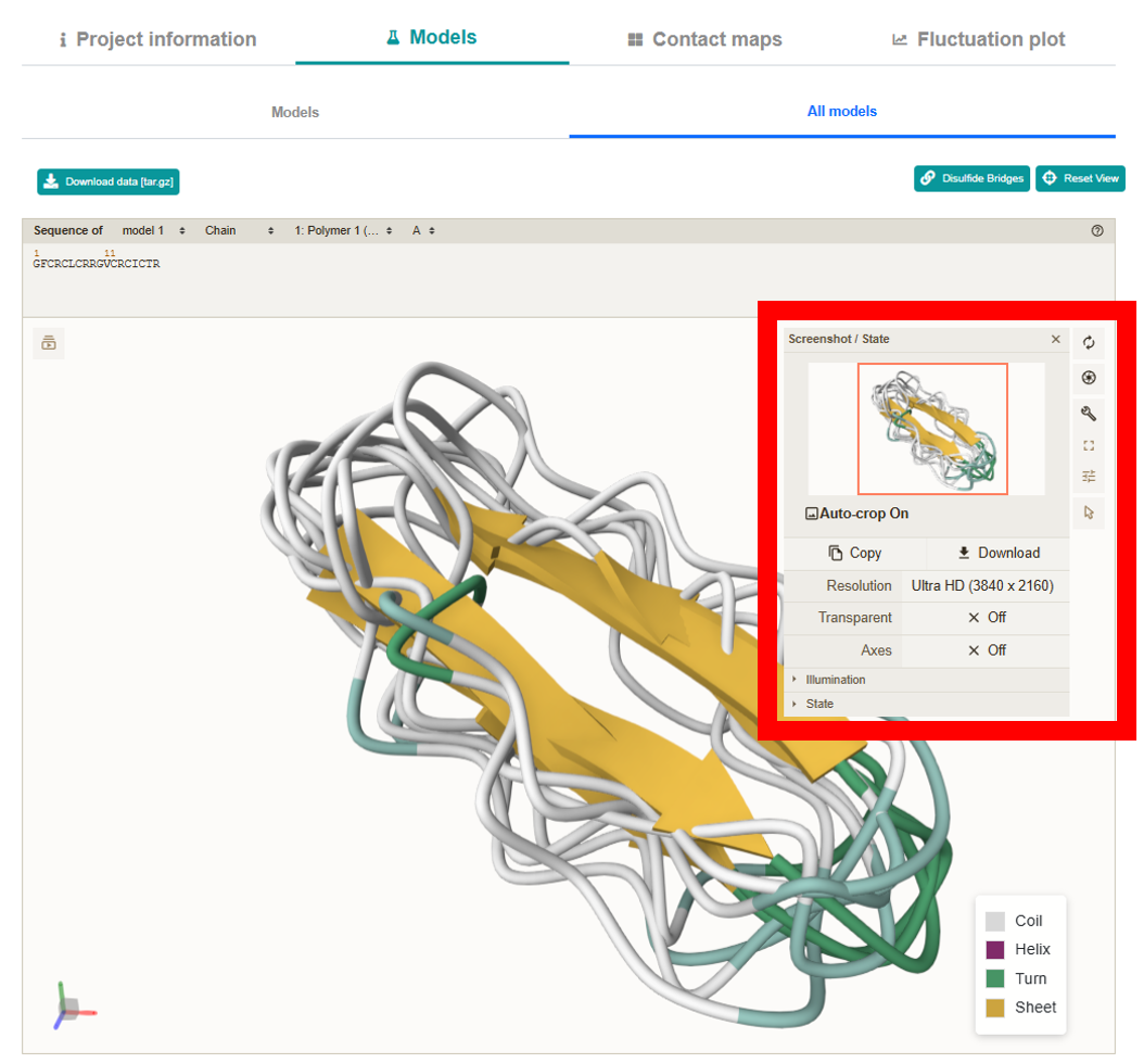
• All models:
  Presents all 10 models simultaneously in a secondary structure representation.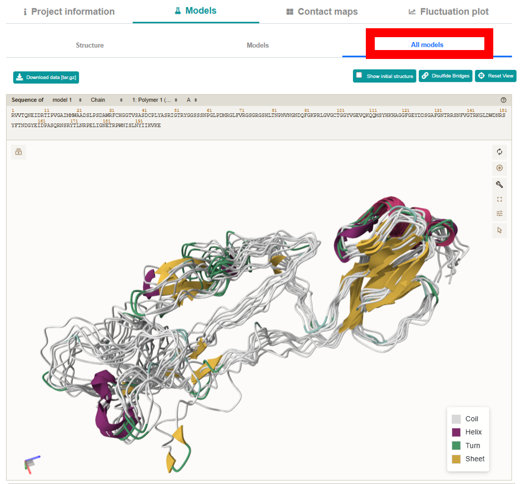

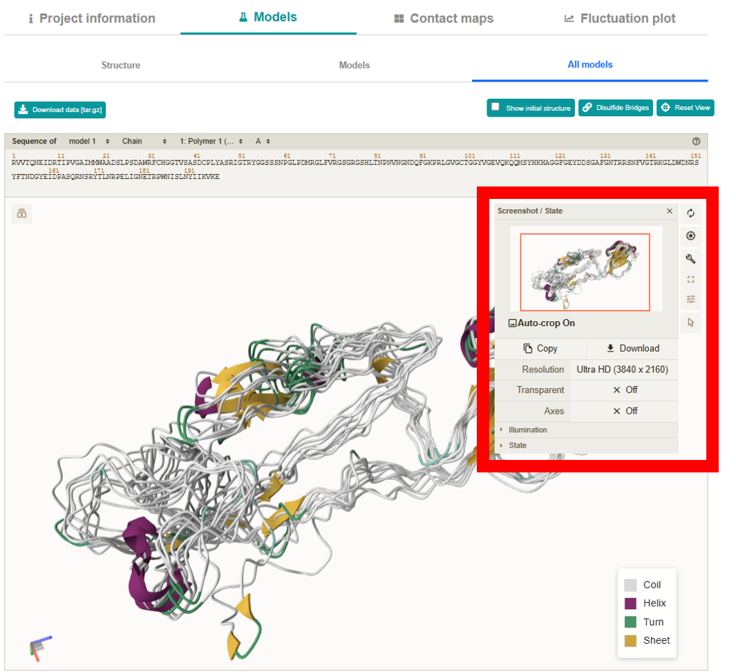
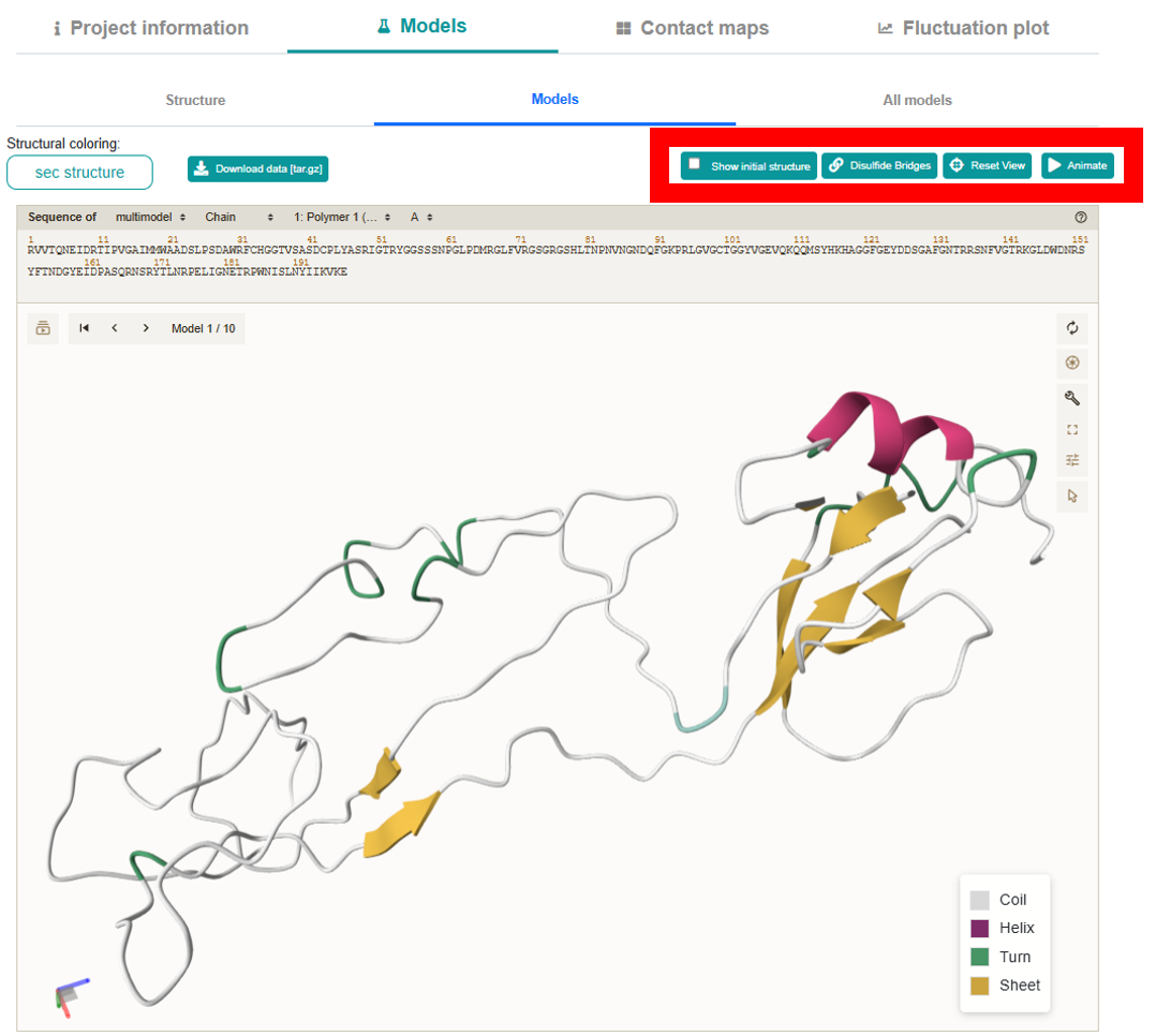Across these sub-tabs, you’ll find buttons to download a tar.gz archive of all output structures, toggle the display of the initial structure (aligned with the current model), show disulfide bridges, reset the view, and—within the Models sub-tab—animate the model sequence in a carousel-like loop. Located on the right side of the viewer, these options allow further customization, including full-screen mode and exporting high-resolution images. 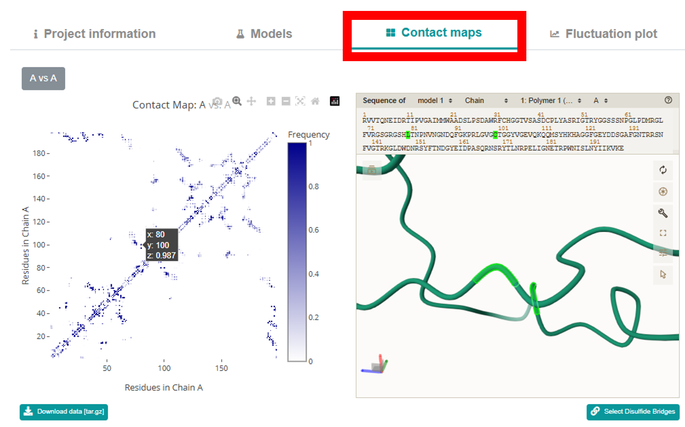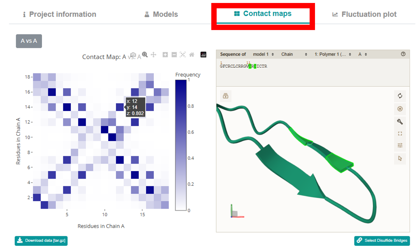Contact Maps section features an interactive Plotly map that lets you examine the interaction interfaces between residues (both inter- and intra-residue contacts). Buttons above the map let you choose the desired contact map, and clicking any contact zooms in on and highlights the corresponding amino acids in the mol* viewer. The map displays residue numbers and contact frequency values on hover, supports zooming, dragging, and can be downloaded as a PNG. Below the map, additional buttons allow you to download a tar.gz archive with the contact map data and to display disulfide bonds. 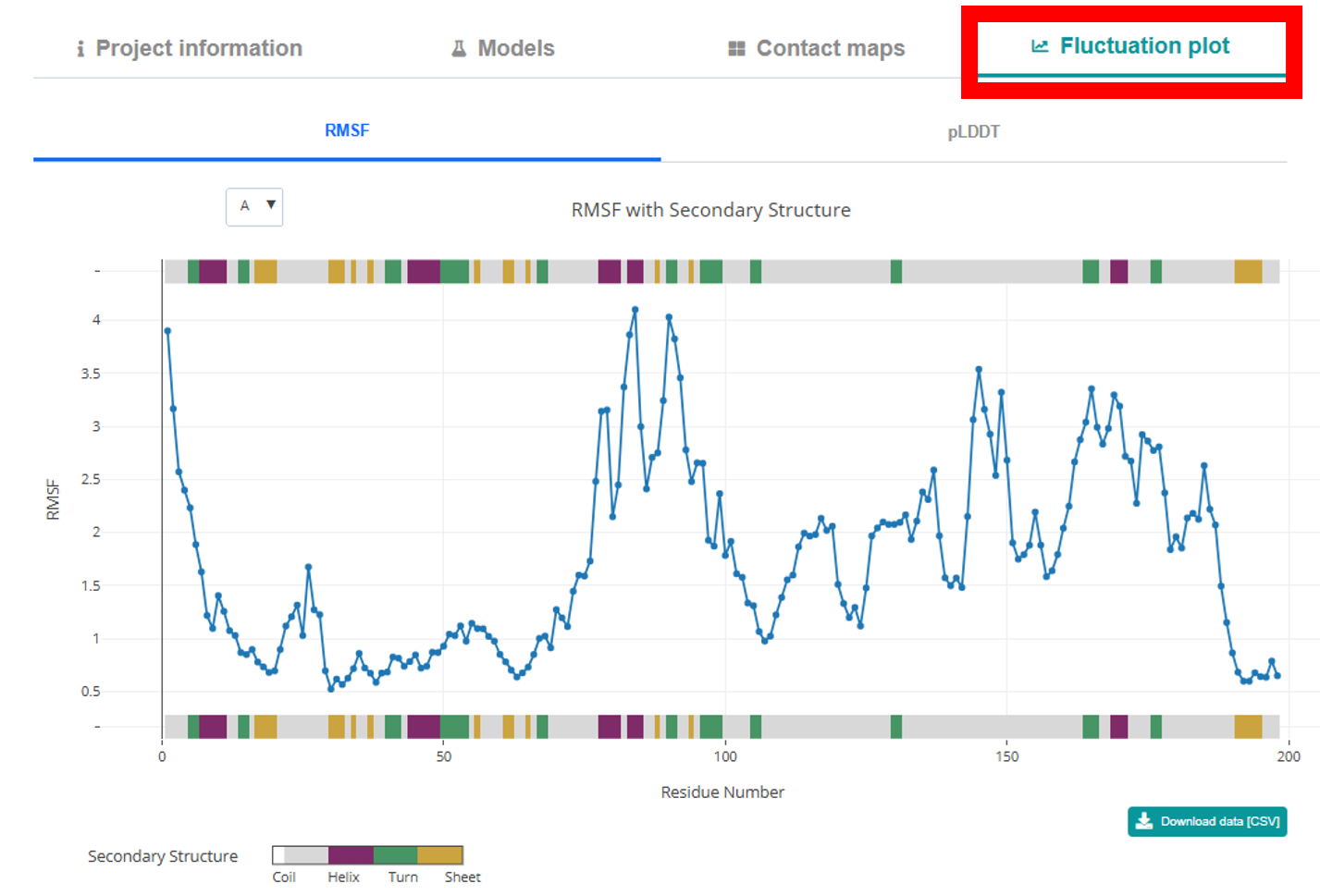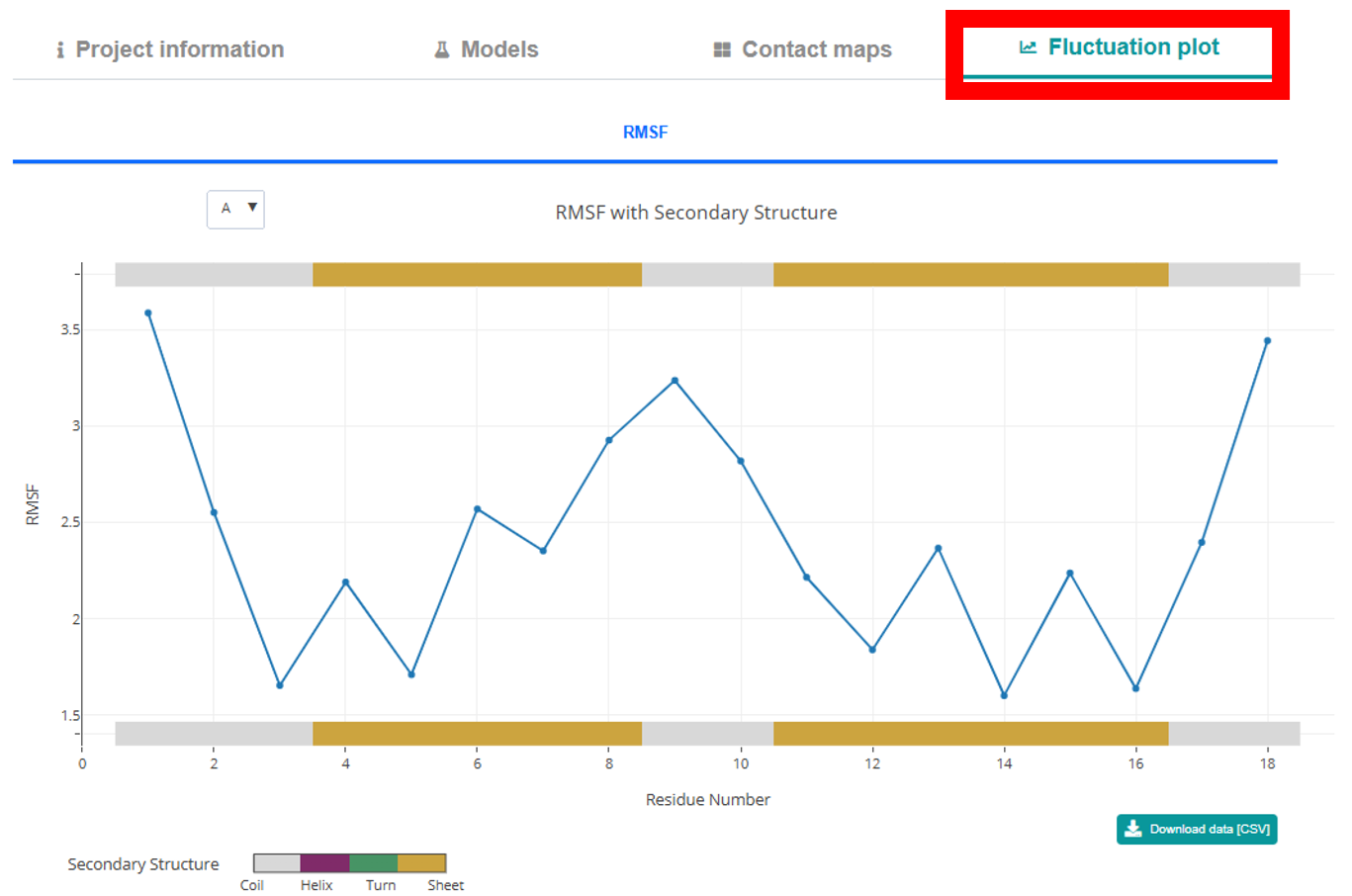Fluctuation Plot Tab. Here you can explore an interactive 2D Plotly plot that charts RMSF versus residue for a selected chain (choosable via a dropdown). The plot is flanked by color-coded secondary structure representations that provide residue and structure details on hover. If available, an option to view a pLDDT plot versus residue is also provided. A CSV download button below the plot allows you to export the RMSF data.

How to analyse peptide modeling?

When you initiate a new job in CABSflex 3.0, the interface starts with a single Project Information tab. This tab is split into two sections: the upper section shows basic project details along with buttons to download the output files, while the lower section provides in-depth details and simulation parameter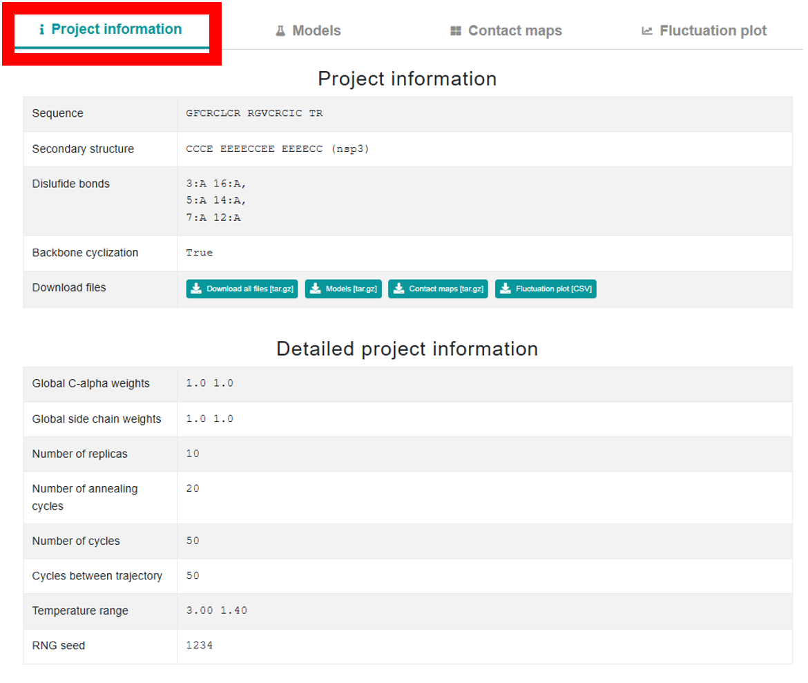s. After job completion, the page expands to include three additional tabs – Models, Contact Maps, and Fluctuation Plot – each designed to help you explore different aspects of the peptide modeling results.

Models section leverages the interactive mol* viewer for 3D visualization and is organized into two sub-tabs:

• Models:
  Loads by default to display each of the 10 output models one at a time with next/previous navigation. It offers a “Structural coloring:” dropdown (allowing you to color the model by sequence, chain, secondary structure, or choose a custom monochrome color via a color picker).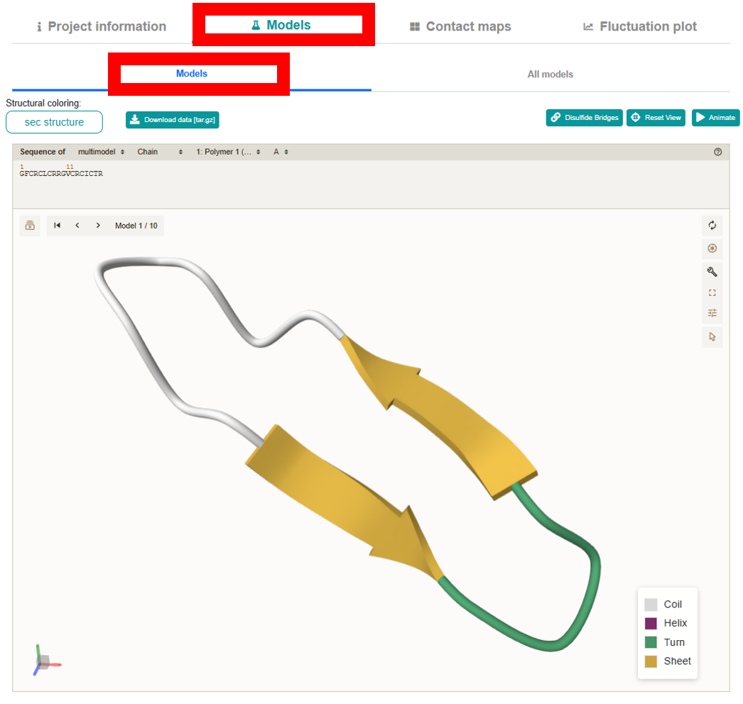
• All models:
  Presents all 10 models simultaneously in a secondary structure representation.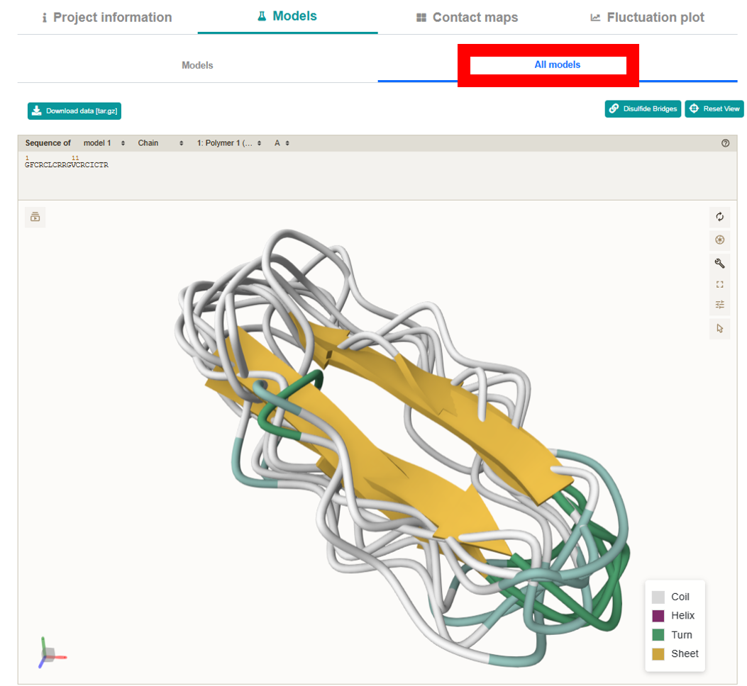

Across these sub-tabs, you’ll find buttons to download a tar.gz archive of all output structures, show disulfide bridges, reset the view, and—within the Models sub-tab—animate the model sequence in a carousel-like loop. Located on the right side of the viewer, these options allow further customization, including full-screen mode and exporting high-resolution images. Contact Maps section features an interactive Plotly map that lets you examine the interaction interfaces peptide residues. Clicking any contact zooms in on and highlights the corresponding amino acids in the mol* viewer. The map displays residue numbers and contact frequency values on hover, supports zooming, dragging, and can be downloaded as a PNG. Below the map, additional buttons allow you to download a tar.gz archive with the contact map data and to display disulfide bonds. Fluctuation Plot Tab. Here you can explore an interactive 2D Plotly plot that charts RMSF versus residue. The plot is flanked by color-coded secondary structure representations that provide residue and structure details on hover. A CSV download button below the plot allows you to export the RMSF data.

What are protein restraints?

Protein restraints are artificial "forces" that keep pairs of residues at specific distances during a simulation. They help control how a protein moves by limiting certain structural changes. The restraints add to the total simulation energy when the distance between restrained residues goes beyond a set limit. During the simulation, if the protein moves in a way that breaks a restraint, the system applies a penalty to push it back within the defined limits.

Before the CABS-flex simulation starts, the server automatically generates distance restraints based on the initial shape of the input structure and the selected Flexibility Mode (How to use flexibility mode?). Users can also add or modify these restraints as needed (How to use advanced simulation options?). The restraint is defined by the following syntax:

"residue1_id residue2_id distance weight”, for example:
“123:A 73:B 12.5 1.0”. This example defines a single restraint between the 123th residue of chain A and the 73rd residue of chain B to be at a distance of 12.5 Å with a restraint weight of 1.0. The higher the restraint weight, the greater the energy penalty.

How to cite CABS-flex 3.0 server?

When you use CABS-flex 3.0, cite the paper:

• CABS-flex 3.0: An Online Tool for Simulating Protein Structural Flexibility and Peptide Modeling - submitted for review

Papers describing some functionalities of CABS-flex 3.0 method:

• Integrating AlphaFold pLDDT Scores into CABS-flex for enhanced protein flexibility simulations Comput Struct Biotechnol J, 23:4350-4356, 2024
  https://doi.org/10.1016/j.csbj.2024.11.047
• Structure prediction of linear and cyclic peptides using CABS-flex Brief Bioinform, 25(2):bbae003, 2024
  https://doi.org/10.1093/bib/bbae003

Review on CABS-flex applications:

• Exploring protein functions from structural flexibility using CABS-flex modeling Protein Sci, 33(9):e5090, 2024
  https://doi.org/10.1002/pro.5090

How to report issues with CABS-flex 3.0 server?

In case of any issues, please report them using the CABS-flex 3.0 issue tracker available at https://github.com/LCBio/cabs-flex/issues.

You can also email us at sekmi@chem.uw.edu.pl